Example 1: Load one file into the Resonator class
By: Faustin Carter, 2016, updated 2018
This notebook imports the data from one Agilent file, creates a
Resonator object, runs a fitting routine, and then plots the data
and fit curves in a nice way.
Once you’ve understood this example, you should be able to replicate it
with your own data simply be writing a custom process_file function
and updating the code that finds the datafile.
#Set up the notebook for inline plotting
%matplotlib inline

#For high-res figures. You can comment this out if you don't have a retina screen
%config InlineBackend.figure_format = 'retina'

#For pretty printing of dicts
import pprint as pp

#Because you should always import numpy!
import numpy as np
Load up the scraps modules
You’ll need to change the path to reflect wherever you stored the code
import os

#Add the scraps folder to the path. You can skip this if you pip installed it.
import sys
sys.path.append(os.getcwd()+'scraps/')

#Load up the resonator code!
import scraps as scr
Load a file and process the data
This unpacks the file data into a dict objects. This block of code is the only thing you need to change to make this work with your data.
The data dict has the following quantities:
I, Q, and freq: numpy arrays of data from the VNA file
name: an arbitrary string describing the resonator. This is description of the physical object. So if you run two sweeps on the same resonator at different powers or temperatures, you should give them the same name.
pwr, temp: floats that describe the power in dB and the temperature in K that the measurement was taken at.
#Load in a file
dataFile = './ExampleData/RES-1_-10_DBM_TEMP_0.113.S2P'

#Use the process_file routine to read the file and create a dict of resonator data
fileDataDict = scr.process_file(dataFile, skiprows=1)

#Look at the contents of the dict:
pp.pprint(fileDataDict)
{'I': array([-0.022739, -0.022687, -0.02265 , ...,  0.063827,  0.063836,
        0.063869]),
 'Q': array([ 0.062457,  0.062449,  0.062447, ...,  0.02939 ,  0.029329,  0.02928 ]),
 'freq': array([  8.17088000e+09,   8.17088400e+09,   8.17088800e+09, ...,
         8.17887200e+09,   8.17887600e+09,   8.17888000e+09]),
 'name': 'RES-1',
 'pwr': -10.0,
 'temp': 0.113}
Make a Resonator object
You can either create a resonator object directly, or use the
makeResFromData helper tool, which takes the data dict you made
earlier as an argument. The makeResFromData tool also allows you to
simultaneously fit the data to a model, by passing the model along.
makeResFromData returns a resonator object, as well as the
temperature rounded to the nearest 5 mK and the power. This is for
convenience when dealing with large numbers of Resonator objects
programmatically.
The Resonator object takes the I, Q, and freq data and calculates
magnitude and phase.
The cmplxIQ_params function sets up a lmfit Parameters
object which can later be passed to a fitting function. It also tries to
guess the baseline of the magnitude and the electrical delay (i.e.
baseline) of the phase, as well as starting values for frequency and
quality factor. The cmplxIQ_fit function is model function that uses
the parameters defined in cmplxIQ_params that is passed to the
do_lmfit or do_emcee methods of the Resonator object.
#Create a resonator object using the helper tool
resObj1 = scr.makeResFromData(fileDataDict)

#Create a resonator object using the helper tool and also fit the data
#To do this, we pass a function that initializes the parameters for the fit, and also the fit function
resObj2 = scr.makeResFromData(fileDataDict, paramsFn = scr.cmplxIQ_params, fitFn = scr.cmplxIQ_fit)

#Check the temperature and power
print('Temperature = ', resObj1.temp)
print('Power = ', resObj1.pwr)

#Check to see whether a results object exists
print('Do fit results exist for the first object? ', resObj1.hasFit)
print('Do fit results exist for the second object? ', resObj2.hasFit)


#Explicitly call the fitter on the first object.
#Here we will call it, and also override the guess for coupling Q with our own quess
resObj1.load_params(scr.cmplxIQ_params)
resObj1.do_lmfit(scr.cmplxIQ_fit, qc=5000)

#Check to see whether a results object exists again, now they are both True
print('Do fit results exist for the first object? ', resObj1.hasFit)
print('Do fit results exist for the second object? ', resObj2.hasFit)

#Compare the best guess for the resonant frequency (minimum of the curve) to the actual fit
#Because we didn't specify a label for our fit, the results are stored in the lmfit_result
#dict under the 'default' key. If we passed the optional label argument to the do_lmfit
#method, it would store the results under whatever string is assigned to label.
print('Guess = ', resObj2.fmin, ' Hz')
print('Best fit = ', resObj2.lmfit_result['default']['result'].params['f0'].value, ' Hz')
print('Best fit with different qc guess = ',
      resObj1.lmfit_result['default']['result'].params['f0'].value, ' Hz')

#You can see the fit is not terribly sensitive to the guess for qc.
Temperature =  0.113
Power =  -10.0
Do fit results exist for the first object?  False
Do fit results exist for the second object?  True
Do fit results exist for the first object?  True
Do fit results exist for the second object?  True
Guess =  8174865993.0  Hz
Best fit =  8174865670.34  Hz
Best fit with different qc guess =  8174865670.34  Hz
Make a pretty plot
Fits aren’t worth anything if you don’t plot the results!!
#When using inline plotting, you have to assign the output of the plotting functions to a figure, or it will plot twice

#This function takes a list of resonators. It can handle a single one, just need to pass it as a list:
figA = scr.plotResListData([resObj1],
                          plot_types = ['LogMag', 'Phase'], #Make two plots
                          num_cols = 2, #Number of columns
                          fig_size = 4, #Size in inches of each subplot
                          show_colorbar = False, #Don't need a colorbar with just one trace
                          force_square = True, #If you love square plots, this is for you!
                          plot_fits = [True]*2) #Overlay the best fit, need to specify for each of the plot_types

Find the maximum liklhood estimate of the fit params using emcee
Let’s use the built-in emcee hooks to compare the results of the
lmfit values with the maximum liklihood values for the fit
parameters.
#Call the emcee hook and pass it the fit function that calculates your residual.
#Since we already ran a fit, emcee will use that fit for its starting guesses.
resObj2.do_emcee(scr.cmplxIQ_fit, nwalkers = 30, steps = 1000, burn=200)
#Check to see that a emcee result exists
print('Does an emcee chain exist? ', resObj2.hasChain)

#Look at the first few rows of the output chain:
chains = resObj2.emcee_result['default']['result'].flatchain

print('\nHead of chains:')
pp.pprint(chains.head())

#Compare withe the mle values (percent difference):
#Maximum liklihood estimates (MLE) are stored in Resonator.mle_vals
#lmfit best fit values for varied parameters are in Resonator.lmfit_vals
diffs = list(zip(resObj2.mle_labels, (resObj2.mle_vals - resObj2.lmfit_vals)*100/resObj2.lmfit_vals))

print('\nPerecent difference:')
pp.pprint(diffs)
Does an emcee chain exist?  True

Head of chains:
             df            f0            qc             qi     gain0  0  88694.637513  8.174866e+09  48825.968684  284032.418900  0.068196
1  88694.633409  8.174866e+09  48825.922210  284032.532886  0.068196
2  88694.633409  8.174866e+09  48825.922210  284032.532886  0.068196
3  88693.936736  8.174866e+09  48825.168106  284030.256892  0.068197
4  88694.084139  8.174866e+09  48825.026661  284031.759541  0.068197

      gain1        gain2    pgain0       pgain1
0  1.040011  1107.766240  1.175713 -1563.868140
1  1.040013  1107.764981  1.175712 -1563.868598
2  1.040013  1107.764981  1.175712 -1563.868598
3  1.040044  1107.745343  1.175714 -1563.867138
4  1.040052  1107.749879  1.175713 -1563.868613

Perecent difference:
[('df', 0.00016457041577626805),
 ('f0', 4.9636793175466591e-09),
 ('qc', -7.1412453256857882e-05),
 ('qi', 0.00066200624835167574),
 ('gain0', -0.00018165545757985608),
 ('gain1', -0.0091685488964723463),
 ('gain2', 0.0047494130464930022),
 ('pgain0', -8.9449361862636539e-05),
 ('pgain1', 0.00025065766561930896)]
Make a sweet giant triangle confusogram of your emcee results.
If you don’t have pygtc installed, open a terminal and type
pip install pygtc. Go ahead, I’ll wait…
import pygtc
#Plot the triangle plot, and overlay the best fit values with dashed black lines (default)
#You can see that the least-squares fitter did a very nice job of getting the values right

#You can also see that there is some strange non-gaussian parameter space that the MCMC
#analysis maps out! This is kind of wierd, but not too worrisome. It is probably suggestive
#that more care is needed in choosing good options for the MCMC engine.

figGTC = pygtc.plotGTC(chains, truths = [resObj2.lmfit_vals])

Notice how the 2D histograms for gain 1 and gain 2 look like
sideways cats eyes? This is probably because the MCMC analsysis hasn’t
quite converged, or maybe there could be outliers. We can plot the
actual chains to see for ourselves.
#We will need to directly use matplotlib for this
import matplotlib.pyplot as plt

#First, let's make a copy of the chains array so we don't mess up the raw data
mcmc_result = resObj2.emcee_result['default']['result'].chain.copy()

#And we can plot the chains to see what is going on
for ix, key in enumerate(resObj2.emcee_result['default']['mle_labels']):
    plt.figure()
    plt.title(key)
    for cx, chain in enumerate(mcmc_result[:,:,ix]):
        plt.plot(chain)
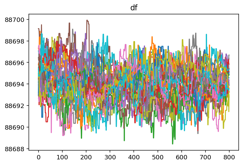

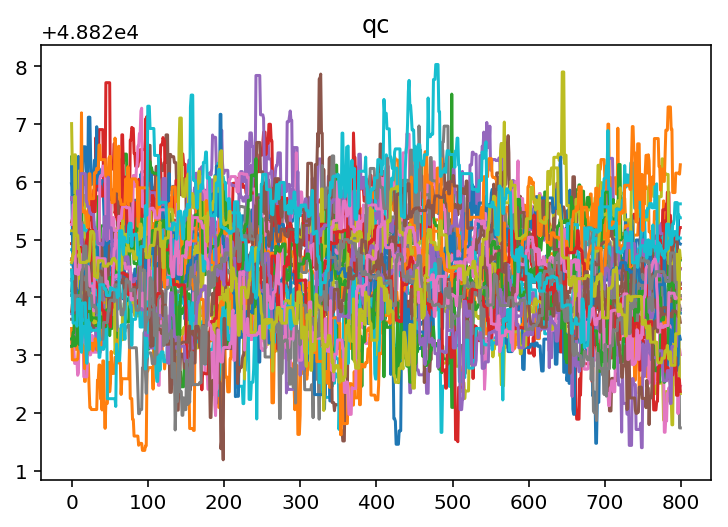

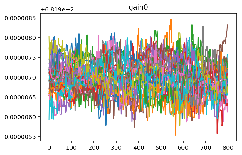

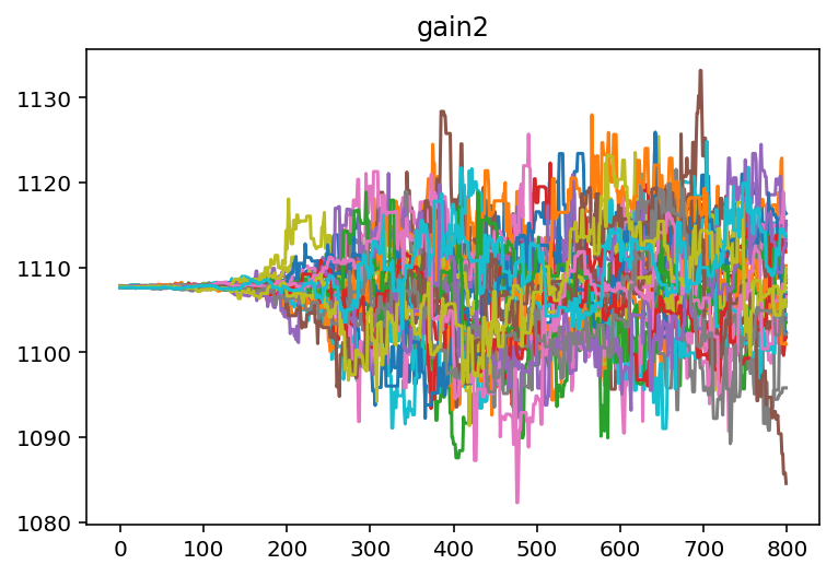

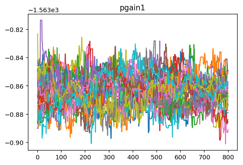
It looks like we need to burn off some samples from the beginning of
each chain so that we are only operating on data that has converged. We
can use a built in method to do this. From looking at the chains for
gain 1 and gain 2 it looks like 400 samples should be about
right.
#Do the burn
resObj2.burn_flatchain(400)

#This will add a new flatchain object, which we can use to plot a new corner plot
pygtc.plotGTC(resObj2.emcee_result['default']['flatchain_burn']);
/Users/fcarter/anaconda/envs/py36/lib/python3.6/site-packages/pandas/core/dtypes/dtypes.py:150: FutureWarning: elementwise comparison failed; returning scalar instead, but in the future will perform elementwise comparison
  if string == 'category':
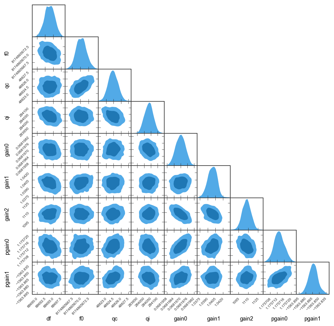
The cat-eye shape is gone now. It looks like there is a little
bi-modality in the df and f0 histograms, but exploring that can
be an exercise for the reader!